Code
library(readxl)
df <- read_excel("_data/LungCapData.xls")Yakub Rabiutheen
September 20, 2022
First, let’s read in the data from the Excel file:
The distribution of LungCap looks as follows:
The histogram suggests that the distribution is close to a normal distribution. Most of the observations are close to the mean. Very few observations are close to the margins (0 and 15).
Comparison of the Genders for both Men and Women using a Boxplot.
Here is the capacity of Smokers vs Non-Smokers
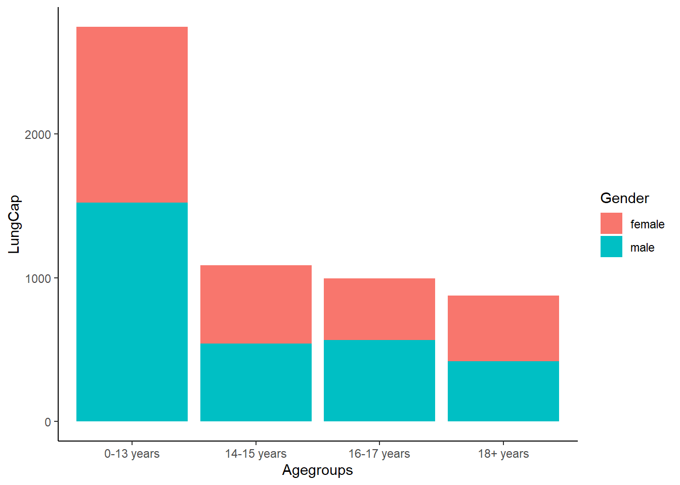
Let’s break it down even further, this is the Lung Capacity by Age Group
Below is the overall Lung Capacity of Age Groups without including Smokers.

#e
Here is a comparision of AgeGroup Lung Capacity in comparison with Smoker vs Non-Smoker.
Based on the comparison of lung capacities between Smoker and Non-Smoker the results are pretty similar.
Question 2
X Frequency
1 0 128
2 1 434
3 2 160
4 3 64
5 4 24As shown below, the most common Prior Convictions is 1.
Dividing by the total among 810 we can determine the probability for each. 810 is the Sum of the Frequency which I checked manually.
Error in mutate(df, Probability = Frequency/sum(Frequency)): could not find function "mutate"Error in eval(expr, envir, enclos): object 'df2' not foundError in df2 %>% filter(X < 2): could not find function "%>%"Error in eval(expr, envir, enclos): object 'b2' not foundError in df2 %>% filter(X <= 2): could not find function "%>%"Error in eval(expr, envir, enclos): object 'c2' not foundFilter for Probability of greater than 2 convictions.
Error in df2 %>% filter(X > 2): could not find function "%>%"Error in eval(expr, envir, enclos): object 'd2' not foundWhat is the expected value of the number of prior convictions?
Error in weighted.mean(df2$X, df2$Probability): object 'df2' not foundError in eval(expr, envir, enclos): object 'e' not foundVariance and Standard Deviation for Question.
---
title: "Homework 1"
author: "Yakub Rabiutheen"
description: "The first homework on descriptive statistics and probability"
date: "09/20/2022"
format:
html:
toc: true
code-fold: true
code-copy: true
code-tools: true
categories:
- hw1
- desriptive statistics
- probability
---
# Question 1
## a
First, let's read in the data from the Excel file:
```{r, echo=T}
library(readxl)
df <- read_excel("_data/LungCapData.xls")
```
The distribution of LungCap looks as follows:
```{r, echo=T}
hist(df$LungCap,freq = FALSE)
```
The histogram suggests that the distribution is close to a normal distribution. Most of the observations are close to the mean. Very few observations are close to the margins (0 and 15).
## b
Comparison of the Genders for both Men and Women using a Boxplot.
```{r}
boxplot(df$LungCap ~ df$Gender)
```
## c
Here is the capacity of Smokers vs Non-Smokers
```{r}
boxplot(df$LungCap~df$Smoke,
        ylab = "Capacity",
        main = "Lung Capacity of Smokers Vs Non-Smokers",
        las = 1)
```
## d
Let's break it down even further, this is the Lung Capacity by Age Group
```{r}
df$Agegroups<-cut(df$Age,breaks=c(-Inf, 13, 15, 17, 20), labels=c("0-13 years", "14-15 years", "16-17 years", "18+ years"))
```
Below is the overall Lung Capacity of Age Groups without including Smokers.
```{r}
library(ggplot2)
ggplot(df, aes(x = LungCap, y = Agegroups, fill = Gender)) +
          geom_bar(stat = "identity") +
          coord_flip() +
          theme_classic()
```
#e
Here is a comparision of AgeGroup Lung Capacity in comparison with Smoker vs Non-Smoker.
```{r}
ggplot(df, aes(x = LungCap, y = Agegroups, fill = Smoke)) +
    geom_bar(stat = "identity") +
    coord_flip() +
    theme_classic()
```
## 1f
Based on the comparison of lung capacities between Smoker and Non-Smoker the results are pretty similar.
```{r}
cov(df$LungCap, df$Age)
cor(df$LungCap, df$Age)
```
Question 2
```{r}
X <- c(0:4)
Frequency <- c(128, 434, 160, 64, 24)
df <- data.frame(X, Frequency)
df
```
As shown below, the most common Prior Convictions is 1.
```{r}
df
```
Dividing by the total among 810 we can determine the probability for each. 810 is the Sum of the Frequency which I checked manually.
```{r}
df2 <- mutate(df, Probability = Frequency/sum(Frequency))
df2
```
B.
Filter for Probability of 2 Convictions
```{r}
b2 <- df2 %>%
  filter(X < 2)
sum(b2$Probability)
```
C.
Filter for Probability of Less than 2 Convictions
```{r}
c2 <- df2 %>%
  filter(X <= 2)
sum(c2$Probability)
```
D.
Filter for Probability of greater than 2 convictions.
```{r}
d2 <- df2 %>%
  filter(X > 2)
sum(d2$Probability)
```
What is the expected value of the number of prior convictions?
```{r}
e <- weighted.mean(df2$X, df2$Probability)
e
```
F.
Variance and Standard Deviation for Question.
```{r}
var(df$X)
```
```{r}
sd(df$X)
```